In the world of digital imagery, where pixels and colors paint a canvas of visual stories, understanding the concept of image histograms is like deciphering an artist’s palette. An image histogram is not just a statistical graph; it’s a visual treasure map that reveals the secrets of an image’s contrast, brightness, and tonal distribution. It’s a tool that photographers, graphic designers, and image-processing algorithms alike rely on to manipulate and enhance the visual content we encounter every day.
Top 10 Free Midjourney Alternatives | Free AI Image Generators
What is DragGAN AI Photo Editor & How to Use It ? For Beginners
Conditional Generative Adversarial Networks (cGANs) Explained
You may be interested in the above articles in irabrod.
But what exactly is an image histogram? In this article, we embark on a journey through the fascinating world of image histograms. We’ll delve into their fundamental nature, explore how they work, and unravel the wealth of information they provide. Whether you’re an aspiring photographer looking to improve your compositions or a data scientist working with image analysis, understanding image histograms is a crucial step towards harnessing the power of visual data. So, let’s begin our exploration into the intricacies of these graphical wonders.
What is an Image Histogram
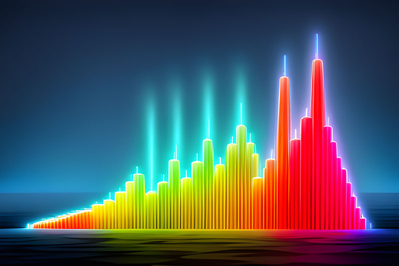
An image histogram is a graphical representation of the distribution of pixel values within a digital image. It provides a visual summary of the tonal distribution of an image, showing how many pixels in the image have each possible intensity value.
In simpler terms, an image histogram illustrates the various shades of gray or colors present in an image and how frequently each of those shades or colors appears. This distribution of pixel values is often used to analyze and manipulate images for various purposes, including adjusting brightness and contrast, enhancing details, and performing image segmentation.
An image histogram typically consists of a horizontal axis representing the range of pixel values (from dark to light) and a vertical axis representing the frequency or number of pixels with each specific value. By examining the peaks, valleys, and overall shape of the histogram, you can gain insights into the image’s tonal characteristics and make informed adjustments to achieve the desired visual effect.
What is an Image Histogram Used For
Image histograms are used for various purposes in image processing and analysis. Here are some common applications:
- Brightness and Contrast Adjustment: Histograms are often used to adjust the brightness and contrast of an image. By stretching or compressing the range of pixel values, you can make an image brighter or darker while maintaining its overall tonal distribution.
- Thresholding: In image segmentation, histograms help determine an appropriate threshold value for separating objects from the background. Pixels with intensity values above or below this threshold can be assigned to different regions or objects.
- Equalization: Histogram equalization is a technique used to enhance the contrast of an image by redistributing the pixel values. This can help reveal details in both dark and light areas of the image.
- Color Correction: For color images, histograms can be analyzed separately for each color channel (e.g., red, green, and blue). Adjusting the histograms of individual channels can correct color balance issues.
- Histogram Matching: Histogram matching involves modifying an image’s histogram to match a specified reference histogram. This is useful for transferring the tonal characteristics of one image to another.
- Noise Removal: Outliers or spurious pixel values can often be identified in a histogram. Removing or smoothing these values can help reduce noise in an image.
- Feature Extraction: In image analysis and computer vision, histograms can be used as features to describe the distribution of pixel intensities in an image. These features can be used for tasks such as object recognition.
- Quality Control: Histogram analysis is also used in quality control processes, such as detecting defects in manufactured products or identifying anomalies in medical images.
- Visualization: Histograms are valuable tools for visualizing the distribution of pixel values within an image. They help users understand the image’s tonal characteristics at a glance.
In summary, image histograms are versatile tools that play a crucial role in various image processing and analysis tasks, from basic adjustments to more advanced applications in fields like computer vision and medical imaging.
Python Image Histogram
Python Image Histogram
CV2
You can use the OpenCV library in Python to compute and visualize image histograms. Here’s a Python code example that demonstrates how to do this:
import cv2
import numpy as np
import matplotlib.pyplot as plt

# Load an image
image_path = 'your_image.jpg'
image = cv2.imread(image_path, cv2.IMREAD_GRAYSCALE)  # Load the image in grayscale

# Calculate the histogram
histogram = cv2.calcHist([image], [0], None, [256], [0, 256])

# Convert the histogram to a 1D array
histogram = histogram.reshape(-1)

# Plot the histogram
plt.figure(figsize=(8, 4))
plt.title("Image Histogram")
plt.xlabel("Pixel Value")
plt.ylabel("Frequency")
plt.xlim([0, 256])  # Set the x-axis limits
plt.plot(histogram, color='black')

# Show the image and histogram
plt.figure(figsize=(10, 5))
plt.subplot(1, 2, 1)
plt.imshow(cv2.cvtColor(image, cv2.COLOR_BGR2RGB))
plt.title("Original Image")
plt.axis("off")

plt.subplot(1, 2, 2)
plt.title("Histogram")
plt.xlabel("Pixel Value")
plt.ylabel("Frequency")
plt.xlim([0, 256])
plt.plot(histogram, color='black')

plt.tight_layout()
plt.show()
In this code:
1. We import the necessary libraries: `cv2` for image processing, `numpy` for array operations, and `matplotlib.pyplot` for plotting.
2. Load an image using `cv2.imread`. We specify `cv2.IMREAD_GRAYSCALE` to load the image in grayscale mode, as histogram computation is typically done on grayscale images.
3. Calculate the histogram using `cv2.calcHist`. The function takes several arguments: the image, a list of channel indices (we use `[0]` for grayscale), a mask (set to `None` for the entire image), the number of bins (256 for pixel values ranging from 0 to 255), and the range of pixel values.
4. Reshape the histogram to a 1D array for plotting.
5. Plot the histogram using `matplotlib.pyplot`. We also display the original image and histogram side by side for visualization.
Make sure to replace `’your_image.jpg’` with the path to the image you want to analyze. This code will display both the image and its histogram for better understanding.
Numpy
You can compute and visualize an image histogram using only `numpy` in Python. Here’s a code example:
import matplotlib.pyplot as plt
import cv2

# Load an image using OpenCV
image_path = 'your_image.jpg'
image = cv2.imread(image_path, cv2.IMREAD_GRAYSCALE)  # Load the image in grayscale

# Compute the histogram using matplotlib
histogram, bins = np.histogram(image.flatten(), bins=256, range=[0,256])

# Plot the histogram
plt.figure(figsize=(8, 4))
plt.title("Image Histogram")
plt.xlabel("Pixel Value")
plt.ylabel("Frequency")
plt.xlim([0, 256])  # Set the x-axis limits
plt.plot(histogram, color='black')

# Show the image and histogram
plt.figure(figsize=(10, 5))
plt.subplot(1, 2, 1)
plt.imshow(cv2.cvtColor(image, cv2.COLOR_BGR2RGB))
plt.title("Original Image")
plt.axis("off")

plt.subplot(1, 2, 2)
plt.title("Histogram")
plt.xlabel("Pixel Value")
plt.ylabel("Frequency")
plt.xlim([0, 256])
plt.plot(histogram, color='black')

plt.tight_layout()
plt.show()
In this code:
1. We load an image using OpenCV (`cv2.imread`) and convert it to grayscale with `cv2.IMREAD_GRAYSCALE`.
2. Compute the histogram using `np.histogram`. We pass the flattened image (converted to a 1D array), the number of bins (256 for pixel values ranging from 0 to 255), and the pixel value range.
3. Plot the histogram using `matplotlib.pyplot`. We also display the original image and histogram side by side for visualization.
Make sure to replace `’your_image.jpg’` with the path to the image you want to analyze. This code will display both the image and its histogram using only `matplotlib`.
Python Only
You can compute an image histogram using only OpenCV (cv2) in Python. Here’s a code example:
import cv2
import numpy as np

# Load an image using OpenCV
image_path = 'your_image.jpg'
image = cv2.imread(image_path, cv2.IMREAD_GRAYSCALE)  # Load the image in grayscale

# Initialize an array to store the histogram
histogram = np.zeros(256, dtype=int)

# Iterate through each pixel in the image and update the histogram
for pixel_value in image.flatten():
    histogram[pixel_value] += 1

# Print the histogram values
for i, count in enumerate(histogram):
    print(f'Pixel value {i}: {count}')

# Optionally, you can visualize the histogram using Matplotlib
import matplotlib.pyplot as plt

plt.figure(figsize=(8, 4))
plt.title("Image Histogram")
plt.xlabel("Pixel Value")
plt.ylabel("Frequency")
plt.xlim([0, 256])  # Set the x-axis limits
plt.plot(histogram, color='black')
plt.show()
Here’s how the code works:
1. Load an image using OpenCV (`cv2.imread`) and convert it to grayscale with `cv2.IMREAD_GRAYSCALE`.
2. Initialize an array called `histogram` to store the histogram. This array has 256 bins to cover all possible pixel values (0 to 255).
3. Iterate through each pixel in the flattened image and update the corresponding bin in the histogram array.
4. Optionally, you can print the histogram values for each pixel value.
5. Finally, you can visualize the histogram using Matplotlib if desired. This code will display a simple line graph representing the image’s histogram.
Replace `’your_image.jpg’` with the path to the image you want to analyze. This code calculates the image histogram using only OpenCV without any additional libraries.
RGB Image Histogram
You can compute an RGB image histogram using OpenCV (cv2) in Python. Here’s a code example:
import cv2
import numpy as np
import matplotlib.pyplot as plt

# Load an image using OpenCV
image_path = 'your_image.jpg'
image = cv2.imread(image_path)

# Split the image into its RGB channels
b, g, r = cv2.split(image)

# Initialize arrays to store the histograms
hist_b = cv2.calcHist([b], [0], None, [256], [0, 256])
hist_g = cv2.calcHist([g], [0], None, [256], [0, 256])
hist_r = cv2.calcHist([r], [0], None, [256], [0, 256])

# Plot the histograms using Matplotlib
plt.figure(figsize=(12, 6))
plt.subplot(131)
plt.title("Blue Histogram")
plt.xlabel("Pixel Value")
plt.ylabel("Frequency")
plt.xlim([0, 256])
plt.plot(hist_b, color='blue')

plt.subplot(132)
plt.title("Green Histogram")
plt.xlabel("Pixel Value")
plt.ylabel("Frequency")
plt.xlim([0, 256])
plt.plot(hist_g, color='green')

plt.subplot(133)
plt.title("Red Histogram")
plt.xlabel("Pixel Value")
plt.ylabel("Frequency")
plt.xlim([0, 256])
plt.plot(hist_r, color='red')

plt.tight_layout()
plt.show()
Here’s how the code works:
1. Load an image using OpenCV (`cv2.imread`).
2. Split the loaded image into its Red, Green, and Blue channels using the `cv2.split` function.
3. Initialize arrays (`hist_b`, `hist_g`, and `hist_r`) to store histograms for each channel separately using `cv2.calcHist`. These histograms will have 256 bins each, covering the range of pixel values from 0 to 255.
4. Plot the histograms using Matplotlib. Each channel’s histogram is plotted in a separate subplot for better visualization.
5. Adjust the titles, labels, and axis limits as needed for clarity.
Replace `’your_image.jpg’` with the path to the RGB image you want to analyze. This code calculates and displays the histograms for the Red, Green, and Blue channels of the image.
Conclusion
In conclusion, an image histogram is a powerful tool for understanding the distribution of pixel values in an image. It provides a visual representation of how frequently each pixel value appears, which can reveal important characteristics of the image, such as its brightness, contrast, and overall tonal range.